Theory and Concepts
In this section, we cover some key concepts, including the reference frames and rigid-body states that CADDEE uses for analyses. This is important informations for users as well as developers that wish to interface their solvers with CADDEE.
Reference frames and rigid-body states
There are currently two main reference frames used in CADDEE, both of which follow the right-hand rule convention.
Inertial reference frame (denoted with subscipt “I”): fixed to the ground with z-axis pointing “up”
Body-fixed reference frame (denoted with subscript “B”): fixed to the system, which is allowed to translate and rotate relative to the inertial reference frame.
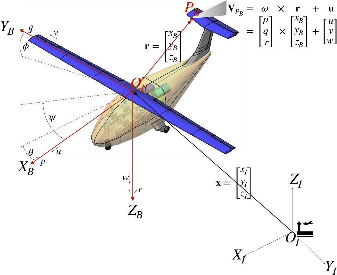
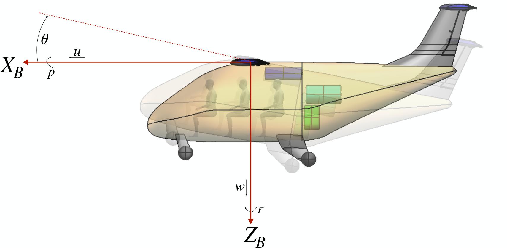
In the figures below, we show an isometric and several 2-D views of the body-fixed (and inertial) reference frame for the case of aircrfat flight-dynamics. By convention, the body-fixed reference frame for aircraft is defined as
X: in the direction of the nose of the aircraft
Y: in the direction of the right wing
Z: downward
Related to the concept of the inertial and body-fixed reference frame are the rigid-body states (also referred to as “aircraft states” in the aircraft design community) that CADDEE uses, which are given by the following 12-dimensional state vector \(\mathbf{s}\)
\(\mathbf{s} = [u, v, w, p, q, r, \phi, \theta, \psi, x, y, z]\),
where \(\mathbf{u} = [u, v, w]\) are the linear velocities, \(\boldsymbol{\omega} = [p, q, r]\) are rotation rates (i.e., angular velocities), and \([\phi, \theta, \psi]\) are the Euler angles corresponding to roll, pitch, and yaw, respectively. These quantities are all taken with respect to the body-fixed reference frame. Lastly, \(\mathbf{x} = [x, y, z]\) are the coordinates of the system (i.e., the origin of the body-fixed frame) with respect to the inertial reference frame.
Isometric view
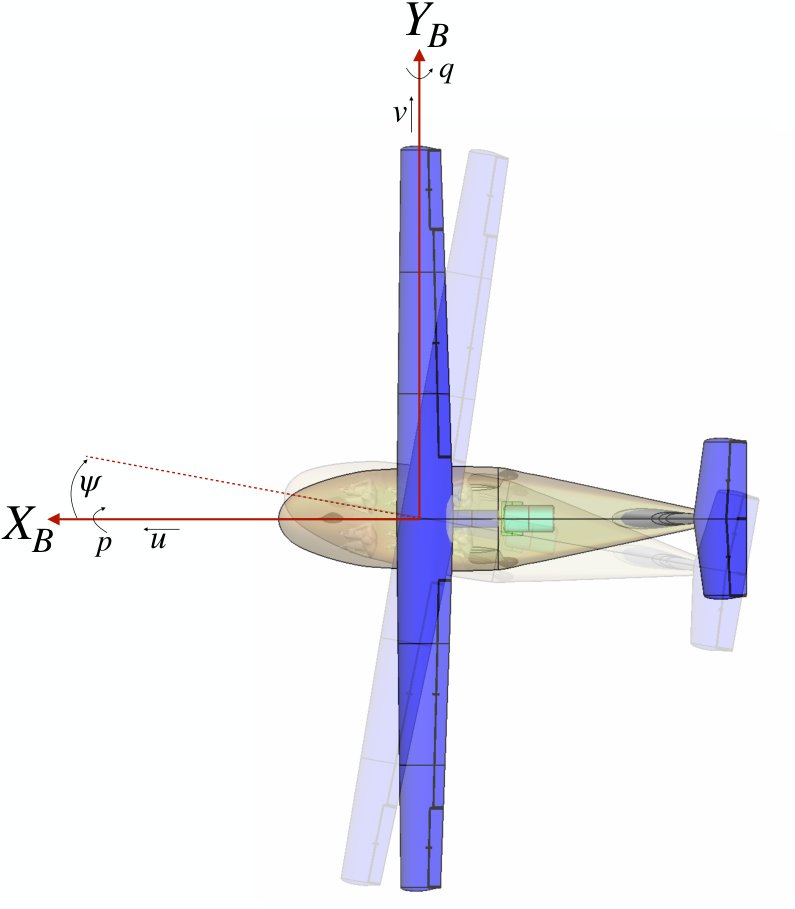
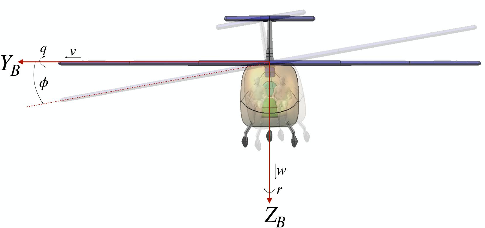
2-D views
Top view |
Front view |
Side view |
|---|---|---|
|
|
|
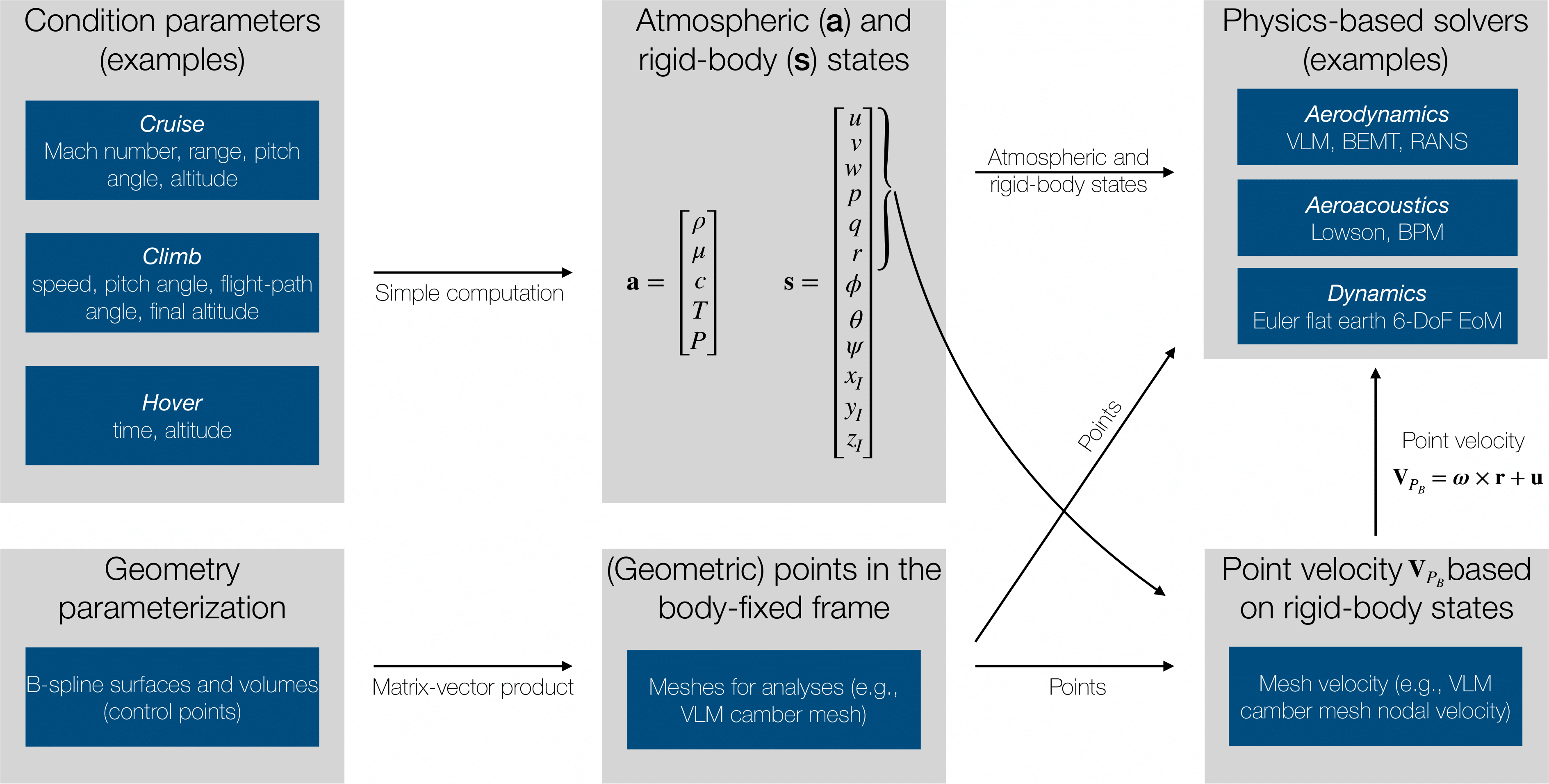
Condition parameterization and solver inputs
Having gone over the reference frames that CADDEE uses, we can now discuss how CADDEE processes information regarding the geometry and conditions. CADDEE will always provide the 12 rigid-body states to a solver in addition to points on the geometry (i.e., meshes). In addition, CADDEE will compute the point velocities (i.e., nodal mesh velocities) in terms of the body-fixed linear and angular velocities as indicated in the diagram. This means that in most cases, a solver does not need to know about or work with the 12-rigid body states, although they are provided in general. For example, after creating a VLM mesh, CADDEE will computate the nodal mesh-velocities, taking into account any rotation rates.
Note
Any solver should return the residual of any non-linear operation in order to be compatible with SIFR along with their explicit outputs/quantities of interest. In addition, certain solvers must output a minimum number of varialbes (with the correct spelling):
Aero-propulsive solver
output_var_group.forces (num_nodes, 3)
output_var_group.moments (num_nodes, 3)
Structural solver
output_var_group.displacements
output_var_group.rotations (if applicable)
Keep in minds that for work conservation (a feature of SIFR), solvers need to also implement an invariant matrix (not currently a requirement). Input and output maps (to the OML) can be defined by the sovler but are not necessary if SIFR’s standard maps are sufficient. Lastly, CADDEE will have default meshing capabilities for standard meshes like VLM mesh or 1-D beam meshes.